This is a fast C++ Voronoi diagram example. The Voronoi diagram (Wikipedia) divides the plane into convex regions around the input points such that each region is closest to one point. There is an incredible number of applications for the Voronoi diagram so many scientists and engineers are familiar with this basic concept.
A C++ Voronoi library must have fast point location, it must be robust to degenerate settings and deal with infinite cells so that it is easy to use. The C++ demo in “examples_2D/ex12_voronoi.cpp” shows that Fade has all these properties. Let’s discuss this example:
A Voronoi diagram in C++
The below code creates a Delaunay triangulation, similarly as in many of the previous examples. But then it fetches its dual graph, the Voronoi diagram:
std::cout<<"* Example12: Voronoi - Point location in a Voronoi diagram"<<std::endl;
// * Step 1 * Create input points (on circles and on a grid). Each
// of these plays two roles: It is a Delaunay-Vertex
// AND a site of one Voronoi cell.
std::vector<Point2> vPoints;
generateCircle( 20,25,75,20,20,vPoints);
generateCircle( 10,25,75,10,10,vPoints);
generateCircle( 20,75,35,10,30,vPoints);
for(double x=0;x<41.0;x+=10)
{
for(double y=0.0;y<41;y+=10)
{
vPoints.push_back(Point2(x+.5,y+.5));
}
}
// * Step 2 * Draw the Voronoi diagram and Delaunay triangulation
// Infinite Voronoi cells are automatically clipped.
Fade_2D dt;
dt.insert(vPoints);
Voronoi2* pVoro(dt.getVoronoiDiagram());
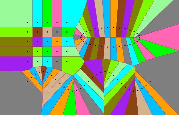
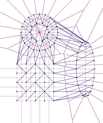
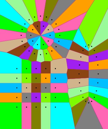
pVoro->show("voronoi_and_delaunay.ps",true,false,true,true,false); // Options: Voro=true,Fill-Colors=false,Sites=true,Delaunay=true,Labels=false
pVoro->show("voronoi_and_sites.ps",true,true,true,false,false); // Options: Voro=true,Fill-Colors=true,Sites=true,Delaunay=false,Labels=false
...- Step 1 creates a few input points lying on a circle and on a grid.
- Step 2 triangulates the input. Afterwards it fetches the Voronoi diagram using
Fade_2D::getVoronoiDiagram()and then makes two postscript visualizations. That’s it, see the resulting images below…
“Hint: If you find it more convenient to deal only with finite Voronoi cells, here’s a simple trick: Compute the bounding box of your sites, inflate the box by factor 10 and then add its 4 corner points to the sites to make all previous cells finite.”
Nearest neighbor search / cell search
The below code snippet finds the Voronoi cell of an arbitrary query point. Then it makes another visualization.
// * Step 3 * Assign arbitrary indices to the Voronoi cells. This
// is completely optional. You can use this feature
// for visualization OR to associate Voronoi cells with
// your own data structures.
std::vector<VoroCell2*> vVoronoiCells;
pVoro->getVoronoiCells(vVoronoiCells);
for(size_t i=0;i<vVoronoiCells.size();++i)
{
VoroCell2* pVoro(vVoronoiCells[i]);
pVoro->setCustomCellIndex(int(i));
}
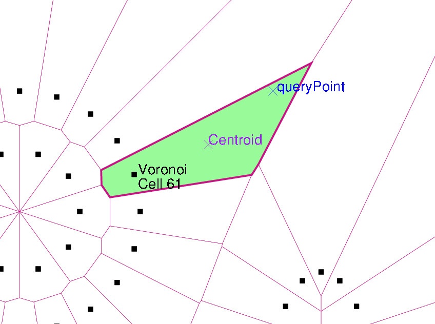
// * Step 4 * Locate the cell of an arbitrary query point.
Point2 queryPoint(67,95);
VoroCell2* pVoroCell(pVoro->locateVoronoiCell(queryPoint));
Visualizer2 v("located_cell.ps");
Bbox2 bbx(dt.computeBoundingBox());
bbx.enlargeRanges(1.5);
v.setLimit(bbx); // Manually set a limit to clip the viewport.
pVoro->show(&v,true,false,true,false,false); // Options: Voro=true,Fill-Colors=false,Sites=true,Delaunay=false,Labels=false
v.addObject(Label(queryPoint," queryPoint"),Color(CBLUE));
if(pVoroCell!=NULL)
{
int cellIdx(pVoroCell->getCustomCellIndex());
std::cout<<"Found the voronoi cell no. "<<cellIdx<<std::endl;
// Color the located cell red
v.addObject(pVoroCell,Color(CPALEGREEN,1.0,true));
// Write a label that shows its custom cell-index
Label l(*pVoroCell->getSite(),
(" Voronoi\n Cell "+toString(cellIdx)).c_str(),false);
v.addObject(l,Color(CBLACK));
Point2 centroid;
double area=pVoroCell->getCentroid(centroid);
if(area<0)
{
std::cout<<"Cell "<<cellIdx<<" is infinite: No area, no centroid"<<std::endl;
}
else
{
std::cout<<"Cell "<<cellIdx<<": area="<<area<<", centroid="<<centroid<<std::endl;
v.addObject(Label(centroid,"Centroid"),Color(CPURPLE));
}
v.writeFile();
}
- Step 3 is optional: It fetches all Voronoi cells and assigns each an arbitrary integer. This is useful to relate the cells with your own data structures. Moreover you can use these integers as labels for a visualization.
- The first two lines in Step 4 locate the Voronoi cell of the query point (x=67.0, y=95.0). The remaining lines from Step 4 draw the diagram again, highlighting the cell. Furthermore, they mark the
site, thecentroidand thequeryPoint.
“Observe that only finite cells have a centroid and a finite area. Fade returns
-1for the area of infinite cells.
“Note: The Voronoi diagram is the dual graph of the Delaunay triangulation. But it is NOT the dual graph of a constrained Delaunay triangulation. Thus, if there are constraint edges in the Delaunay triangulation then you should make them conforming using the method
ConstraintGraph2::makeDelaunay()before using the Voronoi diagram.”
Point location benchmark
The 2D Delaunay Triangulation Benchmark shows that Delaunay triangulations are very fast. Due to the duality constructing a Voronoi diagram is similarly fast. This is important because in many applications the diagram is only beneficial if it can be constructed quickly and if cells can be located quickly. But we must still benchmark nearest neighbor queries, see the code below:
// * Step 5 *   Benchmark mass point location (typ. 0.2 s for 1 mio queries)
std::vector<Point2> vRandomPoints;
generateRandomPoints(1000,0,100,vRandomPoints,1);
Fade_2D dt2;
dt2.insert(vRandomPoints);
Voronoi2* pVoro2(dt2.getVoronoiDiagram());
pVoro2->show("mass_location.ps",true,true,false,false,false);  // Options: Voro=true,Fill-Colors=true,Sites=false,Delaunay=false,Labels=false

timer("massLocate");
for(int i=0;i<1000000;++i)
{
	double x(100.0 * double(rand())/RAND_MAX);
	double y(100.0 * double(rand())/RAND_MAX);
	Point2 q(x,y);
	VoroCell2* pVoroCell(pVoro2->locateVoronoiCell(q));
	unusedValue(pVoroCell); // Avoids an unused-warning
}
timer("massLocate");


return 0;- Step 5 triangulates 1000 points. Afterwards it retrieves the dual graph
pVoro2. Then it enters the “massLocate” timer-section where it finds for 1 million random query points the containing Voronoi cell. This takes only around 0.3 seconds and the time consumption grows only logarithmically in the number of existing cells.
Feel free to link to this site if you find it useful and want to support it!